Paper: DeepSeek-V2: A Strong, Economical, and Efficient Mixture-of-Experts Language Model
Github: DeepSeek-V2
模型结构
模型整体结构: MLA + MoE
- MLA: 在大幅缩小 KV Cache 的同时, 获得超越 MHA 的效果
- MoE: 共 236B 参数, 每个 token 激活 21B 参数
MLA
MHA 在推理阶段的劣势
DeepSeek-V2 对 Transformer 架构中的自注意力机制进行了全方位的创新, 使用 MLA(Multi-head Latent Attention) 结构.
Transformer 标准的 MHA(Multi-Head Attention) 结构中, $n_h$ 为 attention heads 数量, $d_h$ 为每个 head 内部的维度, $\mathbf{h}_t \in \mathbb{R}^d$ 代表了当前 attention layer 层中第 $t$ 个 token 的输入. 标准的 MHA 通过三个不同的参数矩阵 $W_Q,W_K,W_V \in \mathbb{R}^{d_h n_h \times d}$ 得到 $\mathbf{q}_t, \mathbf{k}_t, \mathbf{v}_t \in \mathbb{R}^{d_h n_h}$, 对应于:
$$ \begin{aligned} & \mathbf{q}_t = W_Q \mathbf{h}_t \\ & \mathbf{k}_t = W_K \mathbf{h}_t \\ & \mathbf{v}_t = W_V \mathbf{h}_t \end{aligned} $$
在 MHA 中, $\mathbf{q}_t, \mathbf{k}_t, \mathbf{v}_t$ 被拆分为 $n_h$ 个 heads, 然后每个 head 中进行 attention 计算:
$$ \begin{aligned} & {\left[\mathbf{q}_{t, 1} ; \mathbf{q}_{t, 2} ; \ldots ; \mathbf{q}_{t, n_h}\right]=\mathbf{q}_t,} \\ & {\left[\mathbf{k}_{t, 1} ; \mathbf{k}_{t, 2} ; \ldots ; \mathbf{k}_{t, n_h}\right]=\mathbf{k}_t,} \\ & {\left[\mathbf{v}_{t, 1} ; \mathbf{v}_{t, 2} ; \ldots ; \mathbf{v}_{t, n_h}\right]=\mathbf{v}_t,} \\ & \mathbf{o}_{t, i}=\sum_{j=1}^t \operatorname{Softmax}_j\left(\frac{\mathbf{q}_{t, i}^T \mathbf{k}_{j, i}}{\sqrt{d_h}}\right) \mathbf{v}_{j, i}, \\ & \mathbf{u}_t=W^O\left[\mathbf{o}_{t, 1} ; \mathbf{o}_{t, 2} ; \ldots ; \mathbf{o}_{t, n_h}\right], \end{aligned} $$
每个 head 计算得到的结果再拼接起来, 经过参数矩阵 $W_O \in \mathbb{R}^{d \times d_h n_h}$ 得到 MHA 的输出张量.
在推理阶段, 所有的 keys 和 values 作为 KV Cache, 需要被缓存, 以加速推理. 而根据上式, MHA 结构做 KV Cache, 每个 token 需要缓存 $2n_h d_h l$ 个参数, $l$ 代表 attention layer 数量. MHA 的 KV Cache 量是非常大的, 这会对最大化推理阶段可以支持的 batch size 和 sequence length 是瓶颈.
Low-Rank Key-Value Joint Compression
低秩KV联合压缩(Low-Rank Key-Value Joint Compression)是 MLA 结构的核心, 可以大幅缩小 KV Cache 的占用.
$$ \begin{aligned} \mathbf{c}_t^{K V} & =W^{D K V} \mathbf{h}_t \\ \mathbf{k}_t^C & =W^{U K} \mathbf{c}_t^{K V} \\ \mathbf{v}_t^C & =W^{U V} \mathbf{c}_t^{K V} \end{aligned} $$
$\mathbf{c}_t^{K V} \in \mathbb{R}^{d_c}$ 是压缩后的可训练隐向量, 目标是将 keys 和 values 中的信息压缩进去. $d_c(\ll d_h n_h)$ 代表了隐向量的维度. $W^{D K V} \in \mathbb{R}^{d_c \times d}$ 是输入的下投影矩阵(down-projection matrix), 将输入的维度由 $d$ 压缩到 $d_c$; $W^{U K}, W^{U V} \in \mathbb{R}^{d_h n_h \times d_c}$ 是 keys 和 values 的上投影矩阵(up-projection matrices).
推理过程中, MLA 只需要为每个 token 缓存 $\mathbf{c}_t^{K V}$, 这样每个 token 的 KV Cache 大小减少为 $d_c l$ 个参数.
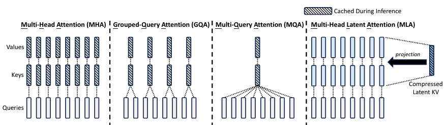
下图对比了常见的 attention 方法 MHA, GQA, MQA 和 MLA 之间在 KV Cache 上的区别. 每个子图代表了某个 token 的计算情况, 所有子图中都有 8 个 heads. 上面这种 KV joint compression 的方法确实可以更进一步地节省 KV Cache 的占用, 虽然在计算量上有增加.
另外为了降低训练过程中 activation 的存储占用, 对 queries 也进行了 low-rank compression, 但这个操作不会降低 KV Cache 的占用, 是为了降低训练时的消耗.
$$ \begin{aligned} \mathbf{c}_t^{Q} & =W^{DQ} \mathbf{h}_t \\ \mathbf{q}_t^C & =W^{U Q} \mathbf{c}_t^{Q} \end{aligned} $$
$\mathbf{c}_t^{Q} \in \mathbb{R}^{d_c^{\prime}}$ 代表了压缩后的隐向量, $d_c^{\prime}(\ll d_h n_h)$ 代表了压缩后隐向量的维度, $W^{DQ} \in \mathbb{R}^{d_c^{\prime} \times d}$, $W^{UQ} \in \mathbb{R}^{d_h n_h \times d_c^{\prime}}$ 分别是下投影和上投影矩阵.
RoPE with MLA
Low-Rank compression 一个最大的问题是与 KV Cache 不兼容. RoPE 需要作用在 queris 和 keys 上, 而作为新的 KV Cache 的 $\mathbf{c}_t^{K V}$ 在计算得到 $\mathbf{k}_t^C$ 之后, 再施加 RoPE, 这样在生成每个 token 时, 都需要对这个 token 之前的所有 token, 都重新计算得到他们的 keys, 这就丧失了 KV Cache 存在的意义, 大幅降低了推理的效率.
为了解决这个问题, 设计了两种不同作用的 queries 和 keys:
- 其中一类 queries 和 keys 不去融合 RoPE, 这些可以完全发挥 Low-Rank compression 的作用
- 另外一类queries 和 keys 去融合 RoPE, 这一类就无法再去使用 Low-Rank compression, 而是采用了 MQA(Multi-Query Attention) 的方式, 所有的 query 共享同一个 keys
这两种 queries 和 keys 在计算 Multi-head attention 之前经过各种计算得到上面的两类, 然后在隐向量维度上拼接起来, 组成一个更长的向量进行 attention 计算. 相当于每个参与 attention 计算的向量, 部分参数包含 RoPE 位置信息, 另外的参数则不包含.
具体来说, 上面使用 Low-Rank compression 得到的 $\mathbf{k}_t^C$ 和 $\mathbf{q}_t^C$ 是不需要计算 RoPE 的 queries 和 keys, 相应的维度为 $d_h n_h$. 另外设置需要计算 RoPE 的 queries 和 keys $\mathbf{q}_{t,i}^{R} \in \mathbb{R}^{d_h^R}$ 和 $\mathbf{k}_t^R \in \mathbb{R}^{d_h^R}$, 其中 $i$ 表示第 $i$ 个 head, $d_h^R$ 代表了这部分每个 head 中的维度.
在使用了上面的方法, 将 MLA 与 RoPE 结合后, 对应的计算过程为:
$$ \begin{aligned} & {\left[\mathbf{q}_{t, 1}^R ; \mathbf{q}_{t, 2}^R ; \ldots ; \mathbf{q}_{t, n_h}^R\right]=\mathbf{q}_t^R=\operatorname{RoPE}\left(W^{Q R} \mathbf{c}_t^Q\right),} \\ & \mathbf{k}_t^R=\operatorname{RoPE}\left(W^{K R} \mathbf{h}_t\right) \text {, } \\ & \mathbf{q}_{t, i}=\left[\mathbf{q}_{t, i}^C ; \mathbf{q}_{t, i}^R\right] \text {, } \\ & \mathbf{k}_{t, i}=\left[\mathbf{k}_{t, i}^C ; \mathbf{k}_t^R\right] \text {, } \\ & \mathbf{o}_{t, i}=\sum_{j=1}^t \operatorname{Softmax}_j\left(\frac{\mathbf{q}_{t, i}^T \mathbf{k}_{j, i}}{\sqrt{d_h+d_h^R}}\right) \mathbf{v}_{j, i}^C \\ & \mathbf{u}_t=W^O\left[\mathbf{o}_{t, 1} ; \mathbf{o}_{t, 2} ; \ldots ; \mathbf{o}_{t, n_h}\right], \end{aligned} $$
可以看到, 每个 head 中计算 RoPE 的 query $\mathbf{q}_{t,i}^{R}$ 和 $\mathbf{k}_t^R$ 的维度都是 $d_h^R$, 而 query 是每个 head 都有, 但 key 是所有 heads 中的 queries 中共享同一个 $\mathbf{k}_t^R$, 是标准的 MQA 思路.
$\mathbf{q}_{t, i}^C ; \mathbf{q}_{t, i}^R$ 两种 query 拼接在一起得到新的 query, $\mathbf{k}_{t, i}^C ; \mathbf{k}_t^R$ 两种 key 拼接在一起得到新的 key, 也能明显看到, key 的一部分是 MHA 的思路, 使用了 Low-Rank compression, 另一部分是所有 head 中拼接相同的 key, 使用了 MQA 的思路.
KV Cache 最终大小
从上面两节可以看到, MLA 是一种 MHA 和 MQA 之间的均衡:
- MHA 部分对应的 $\mathbf{k}_t^C \in \mathbb{R}^{d_h n_h}$ 在上面分析了, 缓存的是 $\mathbf{c}_t^{K V}$, $\mathbf{c}_t^{K V}$ 其实也是所有 head 共用的, 是经过 $W^{U K}$ 得到了 attention 计算各个 head 对应的 keys $\mathbf{k}_t^C = \left[\mathbf{k}_{t, 1}^R ; \mathbf{k}_{t, 2}^R ; \ldots ; \mathbf{k}_{t, n_h}^R\right]$
- MQA 部分引入的 $\mathbf{k}_t^R$ 是需要被缓存的, 这部分包含了 RoPE 的位置信息
因此整个 MLA 机制需要缓存的内容为 $\mathbf{c}_t^{K V} \in \mathbb{R}^{d_c}$ 和 $\mathbf{k}_t^R \in \mathbb{R}^{d_h^R}$, 这样每个 token 对应的 KV Cache 为 $(d_c + d_h^{R})l$ 个元素.
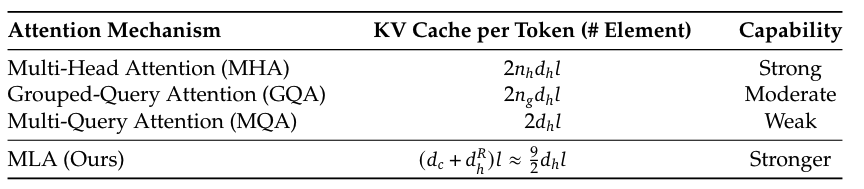
下图是 MHA, GQA, MQA, MLA 四种 attention 机制的 KV Cache 的对比. 参考开源的 DeepSeek-V2 模型中的 config, 可以得到 heads 数量为 $n_h = 128$, head_dim $d_h=128$. 而 MLA 对应的参数为 $d_c=512$, $d_h^R=64$. 可以得到 MLA 中每个 token 对应的 cache 大小为 $(512 + 64)l = \frac{9}{2} \times 128 l = \frac{9}{2} d_h l$, 这个大小介于 MHA 的 $256 d_h l$ 与 MQA 的 $2 d_h l$ 之间. 与 GQA 相比, 相当与 group 数量 $n_g = 2.25$ 大小.
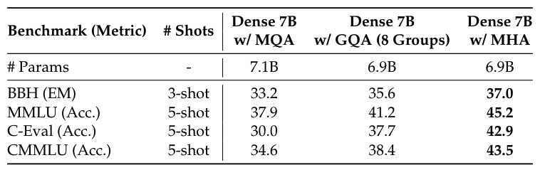
消融实验设计了两组, 分别是 MHA, GQA, MQA 这三种传统方案的对比, 以及 MHA 和 MLA 这两种方案的对比.
在 MHA, GQA, MQA 对比的消融实现中, 使用 7B 大小的模型, 在 1.33T tokens 上分别进行训练得到. 下表中很明显, MHA 是显著由于另外两种方案.
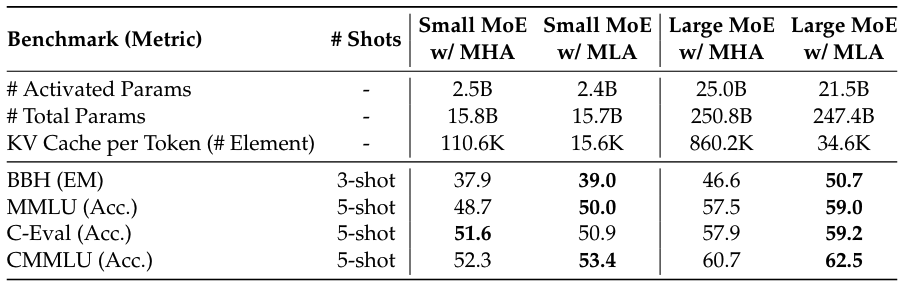
再对比 MHA 和 MLA. 结合 MoE 架构, 在 16B 总参数规模和 250B 总参数规模进行了实验, 对比结果如下表, 在显著降低 KV Cache 的情况下(Small MoE 中 MLA 的 cache 大小为 MHA 的 14%, Large MoE 中为 4%), 基本上在各个 benchmark 上, MLA 都明显超越了 MHA.
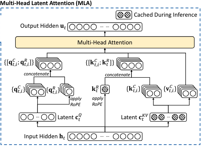
MLA 的完整过程
MLA 中, 第 $t$ 个 token 在 attention 结构中完整的计算过程如下:
$$ \begin{aligned} & \mathbf{c}_t^Q=W^{D Q} \mathbf{h}_t, \\ & {\left[\mathbf{q}_{t, 1}^C ; \mathbf{q}_{t, 2}^C ; \ldots ; \mathbf{q}_{t, n_h}^C\right]=\mathbf{q}_t^C=W^{U Q} \mathbf{c}_t^Q ,} \\ & {\left[\mathbf{q}_{t, 1}^R ; \mathbf{q}_{t, 2}^R ; \ldots ; \mathbf{q}_{t, n_h}^R\right]=\mathbf{q}_t^R=\operatorname{RoPE}\left(W^{Q R} \mathbf{c}_t^Q\right) \text {, }} \\ & \mathbf{q}_{t, i}=\left[\mathbf{q}_{t, i}^C ; \mathbf{q}_{t, i}^R\right] \text {, } \\ & \mathbf{c}_t^{K V}=W^{D K V} \mathbf{h}_t \text {, } \\ & {\left[\mathbf{k}_{t, 1}^C ; \mathbf{k}_{t, 2}^C ; \ldots ; \mathbf{k}_{t, n_h}^C\right]=\mathbf{k}_t^C=W^{U K} \mathbf{c}_t^{K V},} \\ & \mathbf{k}_t^R=\operatorname{RoPE}\left(W^{K R} \mathbf{h}_t\right), \\ & \mathbf{k}_{t, i}=\left[\mathbf{k}_{t, i}^C ; \mathbf{k}_t^R\right], \\ & {\left[\mathbf{v}_{t, 1}^C ; \mathbf{v}_{t, 2}^C ; \ldots ; \mathbf{v}_{t, n_h}^C\right]=\mathbf{v}_t^C=W^{U V} \mathbf{c}_t^{K V},} \\ & \mathbf{o}_{t, i}=\sum_{j=1}^t \operatorname{Softmax}_j\left(\frac{\mathbf{q}_{t, i}^T \mathbf{k}_{j, i}}{\sqrt{d_h+d_h^R}}\right) \mathbf{v}_{j, i^{\prime}}^C \\ & \mathbf{u}_t=W^O\left[\mathbf{o}_{t, 1} ; \mathbf{o}_{t, 2} ; \ldots ; \mathbf{o}_{t, n_h}\right], \end{aligned} $$
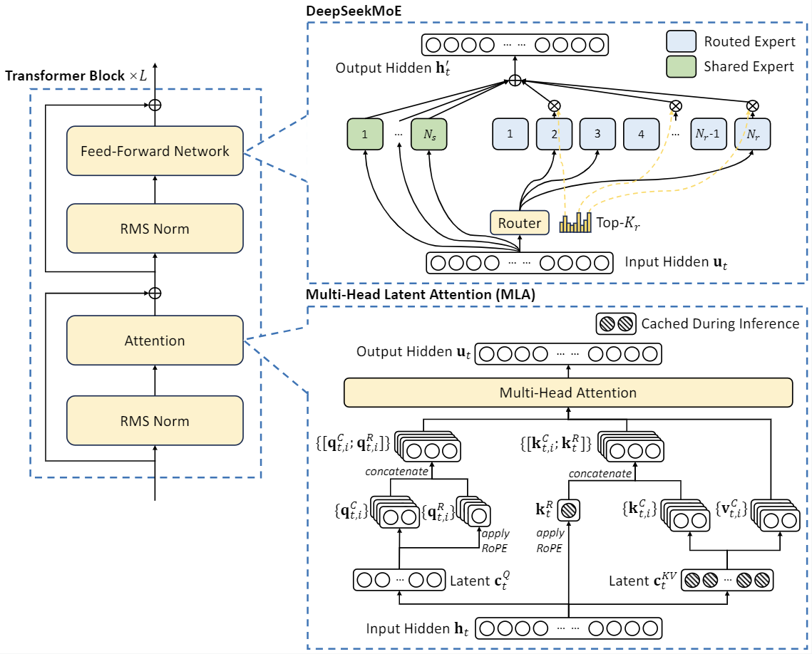
对应的流程图如下(这图真的清晰, 每个张量的 head 情况都准确描述):
代码
具体的细节还是要看代码. 从上面的公式中很明显可以看到引入了很多的权重参数$W$. 首先我们先定义下各个大小参数, 结合开源的 DeepSeek-V2 模型中的 config 中的数值:
hidden_size: 本层输入的大小, 对应上面的 $d$, 值为 5120num_heads: head 数量, 对应 $n_h$, 值为 128q_lora_rank: queries 进行 low-rank compression 后的维度, 对应 $d_c^{\prime}$, 值为 1536qk_nope_head_dim: query 中进行 low-rank compression 不需要进行 RoPE 的维度, 相当于原始的 head 内的维度, 对应 $d_h$, 值为 128qk_rope_head_dim: query 中进行 RoPE 的维度, 对应 $d_h^R$, 值为 64q_head_dim: query 拼接后的维度, 对应 $d_h + d_h^R$, 值为 128 + 64kv_lora_rank: keys 进行 low-rank compression 后的维度, 对应 $d_c$, 值为 512v_head_dim: values 对应的维度, 即原始的 head 内的维度, 对应 $d_h$, 值为 128
在代码中, 关于 query 和 key 这部分定义了 4 个参数权重变量, MLA 引入的各种权重参数, 可以看做通过各种拼接组合, 最终形成了这 4 个变量:
q_a_proj:(hidden_size, q_lora_rank), 即 $(d, d_c^{\prime})$. 这个权重对应的就是公式中的 $W^{DQ} \in \mathbb{R}^{d \times d_c^{\prime}}$, 将输入 $\mathbf{h}_t$ 映射为低秩压缩后的 $\mathbf{c}_t^Q$q_b_proj:(q_lora_rank, num_heads * q_head_dim), 即 $(d_c^{\prime}, n_h \times (d_h + d_h^R))$, 对应的权重为 $W^{UQ} \in \mathbb{R}^{n_h d_h \times d_c^{\prime}}$ 和 $W^{QR} \in \mathbb{R}^{n_h d_h \times d_h^{R}}$, 两个权重分别将低秩压缩后的 $\mathbf{c}_t^Q$ 转化为每个 heads 中不同的两种 queries 成分, 部分经过 RoPE 后再拼接得到最终的 querieskv_a_proj_with_mqa:(hidden_size, kv_lora_rank + qk_rope_head_dim), 即 $(d, d_c + d_h^R)$, 对应的权重为 $W^{DKV} \in \mathbb{R}^{d \times d_c}$ 和 $W^{KR} \in \mathbb{R}^{d \times d_h^R}$, 两个权重分别将输入 $\mathbf{h}_t$ 转化为公共的两种 cache, $\mathbf{c}_t^{K V} \in \mathbb{R}^{d_c}$ 和 $\mathbf{k}_t^R \in \mathbb{R}^{d_h^R}$kv_b_proj:(kv_lora_rank, num_heads * (qk_nope_head_dim + v_head_dim)), 即 $(d_c, n_h \times (d_h + d_h))$, 对应的权重为 $W^{UK} \in \mathbb{R}^{d_c \times n_h d_h}$ 和 $W^{UV} \in \mathbb{R}^{d_c \times n_h d_h}$, 其中 $W^{UK}$ 是将不进行 RoPE 的 keys 部分还原出来, 作为每个 heads 中的 keys 的一部分成分, 与上面得到的 $\mathbf{k}_t^R$ 拼接得到最终的 keys; $W^{UV}$ 是将 KV cache 中的 values 还原出来 使用到的矩阵 相比于 MHA 用到的三个 $(d, n_h d_h)$ 矩阵, 将输入 $\mathbf{h}_t$ 转换成 queries, keys, values, 由于降秩压缩的存在, attention 结构的参数量有减少.
| |
前向传播过程的代码如下, 可以与公式中的过程一一对应.
| |
MoE
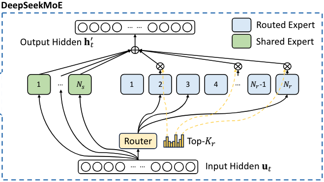
在 FFN 层中, 使用了 DeepSeekMoE 结构. DeepSeekMoE 中将 experts 划分为了两类:
- Routed Expert: 这部分专家负责更准确地获取专业知识
- Shared Expert: 这部分专家负责减少 Routed Expert 之间的知识冗余情况
对于每一个 token, 所有的 Shared Expert 都会被激活, 除此之外再根据 gate 选择 TopK 的 Routed Expert 激活, 将这些专家的输出汇总得到这个 token 最终的输出. 整个过程如下图所示.
$$ \begin{aligned} & \mathbf{h}_t^{\prime}=\mathbf{u}_t+\sum_{i=1}^{N_s} \operatorname{FFN}_i^{(s)}\left(\mathbf{u}_t\right)+\sum_{i=1}^{N_r} g_{i, t} \operatorname{FFN}_i^{(r)}\left(\mathbf{u}_t\right), \\ & g_{i, t} = \begin{cases} s_{i, t}, & s_{i, t} \in \operatorname{Topk}\left(\left\{s_{j, t} \mid 1 \leqslant j \leqslant N_r\right\}, K_r\right), \\ 0, \quad \text { otherwise, }\end{cases} \\ & s_{i, t}=\operatorname{Softmax}_i\left(\mathbf{u}_t^T \mathbf{e}_i\right), \end{aligned} $$
公式化表述:
$\mathbf{u}_t$ 是第 $t$ 个 token 的 FFN 输入, $N_s$ 和 $N_r$ 分别代表 Shared Expert 和 Routed Expert 的数量, $\operatorname{FFN}_i^{(s)}(\cdot)$ 和 $\operatorname{FFN}_i^{(r)}(\cdot)$ 分别代表了第 $i$ Shared Expert 和第 $i$ 个 Routed Expert.
$K_r$ 代表了要激活几个 Routed Expert. $g_{i,t}$ 代表了第 $i$ 个 Routed Expert 对应的 gate value.
$s_{i,t}$ 代表了当前第 $t$ 个 token 对第 $i$ 个 Routed Expert 的倾向程度, 由每个 Routed Expert 对应的 softmax 得到. $\mathbf{e}_i$ 是这层中第 $i$ 个 Routed Expert 对应的 centroid 向量.
最后将选择出的 TopK Routed Expert 乘上对应的 $g_{i,t}$ gate value 作为权重, 再加上所有 Shared Expert 的输入, 以及原始输入 $\mathbf{u}_t$, 得到第 $t$ 个 token 的最终输出 $\mathbf{h}_t^{\prime}$.
在开源的 DeepSeek-V2 模型中的 config 中对应的 Routed Expert n_routed_experts 数量为 160, 选取 num_experts_per_tok TopK $K_r = 6$; Shared Expert 的数量 n_shared_experts 为 2.
代码
其中还是有很多细节, 需要代码阐释. 首先是 MoE 的整体是怎么定义的. 其中通过 config.ep_size 的配置定义了 expert parallel 的数量, 即针对 expert 是否并行计算, DeepSeekMoE 结构进行了专门的优化.
| |
我们只看非并行部分, 作为理解. num_experts_per_tok 定义了每个 token 用几个 router expert. Router experts 中实际上为一个个 DeepseekV2MLP, 这个就是使用了 SwiGLU 激活函数的 MLP 结构.
| |
然后定义了 MoE 需要的 Gate 结构, 后面展开. 然后定义了 Shared experts. 可以看到是使用了一个大的 DeepseekV2MLP 结构作为所有 Shared experts 的汇总. 如果 shared experts 的数量增加, MLP 结构的 intermediate_size 会成比例的增大.
| |
计算过程. 首先接收 hidden_states 作为输入. 将输入传入到 gate 结构中, 得到 topK router experts 对应的 index topk_idx, 以及对应的权重分数 topk_weight.
| |
MoEGate
在 MoEGate 中, 一个 batch 内, 每个样本中的每个 token 都会选择出它对应的 topk 的 router experts. MoEGate 初始化, 声明了一个可训练的 centroid 参数矩阵 weight, 每个 router expert 对应一个向量, 因此 centroid 矩阵的大小为 (n_routed_experts, gating_dim), gating_dim 实际上为 hidden_size 大小.
| |
在前向传播阶段, 输入 hidden_states 为 (b, s, hidden_size), 将输入通过 weight 映射为 (b, s, n_routed_experts), 即 batch 内, 每个样本中的每个 token 对应在所有 router expert 的 logits 分数, 之后进行 softmax 得到归一化的分数.
| |
之后挑选出 topk 的 experts 和对应的分数. 这里有两种策略: gready 和 group_limited_greedy. gready 的方法很简单, 直接使用 topk 函数, 选出 batch 内每个 token 对应的 topk index 以及对应的分数 topk_idx 和 topk_weight, 两个张量的维度为 (b, s, top_k).
| |
而根据配置文件, deepseek-v2 默认的方法为 group_limited_greedy. 在这种方法下, router experts 不再是完全平等竞争, 而是分成了几组, 首先每个组选出代表, 组间进行竞争, 淘汰点所有落后组及其对应的 experts, 再在剩余的组中选择出 topk 的 experts. 在 DeepSeek-V2 的 config 中, 分成了 n_group = 8 组, 总共要选出 topk_group = 3 个组, 然后在这 3 个组的所有 experts 中选举组最优的 num_experts_per_tok = 6 个 experts.
分组的方法, 是将最后一维 n_routed_experts 通过 view 方法转换成 (n_group, n_routed_experts // n_group), 并且将 (b, s) 碾平, 记 b * s = n. 首先得到每个 token 每个 group 的最大分数 group_scores: (n, n_group).
然后根据分数, 选取每个 token 对应的 topk 个组的 index group_idx: (n, topk_group).
然后根据得到的 index 创建 group 的 mask 矩阵, 矩阵的大小为 (n, n_group), 值为 1 代表这个 group 是被选择为 top group 的组, 为 0 代表非 top group, 后面不再使用. 这一步是通过 scatter_ 方法实现的, 得到 group_mask: (n, n_group).
之后, 要根据得到的 top group, 将这些组内所有的 expert 选择出来, 后面在做比较. 方法是根据得到的 group_mask 得到所有 expert 对应的 expert mask, 这里是 score_mask: (n, n_routed_experts). 方法是将 group_mask 扩展 n_routed_experts // n_group 遍, 这样 group_mask 的值就映射到了组内所有的 expert 上, 然后将 mask 矩阵的形状调整为需要的形式. 使用了 unsqueeze, expand, reshape 方法.
得到了 expert mask 之后, 将这个 mask 矩阵覆盖到之前得到的每个 expert 的分数, 挑选出 top group 对应的所有 experts, 在选出这其中的 topk 个 experts.
| |
将 topk 对应的 weights 进行归一化调整.
| |
接下来, DeepSeek-V2 引入了 Expert-Level Balance Loss 的概念, 用在训练阶段, 目的是避免 routing collapse 现象, 即所有 tokens 只激活一部分 experts, 另外一部分 experts 很少被激活, 导致参数效率低下.
Expert-Level Balance Loss 的定义为
$$ \begin{aligned} \mathcal{L}_{\mathrm{ExpBal}}& =\alpha_{1}\sum_{i=1}^{N_{r}}f_{i}P_{i}, \\ &f_{i} =\frac{N_{r}}{K_{r}T}\sum_{t=1}^{T}\mathbb{1}(\mathrm{Token~}t\mathrm{~selects~Expert~}i), \\ &P_{i} =\frac{1}{T}\sum_{t=1}^{T}s_{i,t}, \end{aligned} $$
$s_{i,t}$ 代表的就是第 $i$ 个 router expert 在第 $t$ 个 token 上的分数, 将所有 token 的分数平均, 得到这个 expert 对应的分数 $P_i$. $f_i$ 是第 $i$ 个 expert 对应的 loss 权重, 与 batch 内有多少个 token 激活了这个 expert 相关, 越多的 tokens 选择这个 expert, 则这个 expert 产生的 loss 越大.
最后将分数 $P_i$ 和权重 $f_i$ 乘在一起, expert 的得分越高, 或者这个选择 expert 的 tokens 越多, 说明这个 expert 越有被偏向的风险. 通过 Expert-Level Balance Loss 这个正则项, 来缓解这个问题.
$\alpha_1$ 是这个 loss 的平衡参数.
| |
MoE forward
| |
接下来产生了训练阶段和推理阶段的分歧. 首先看训练阶段.
hidden_states 转换为 (b * s, hidden_size). 首先将其重复 num_experts_per_tok 次, 得到 (b * s * num_experts_per_tok, hidden_size). flat_topk_idx: (b * s * num_experts_per_tok,) 由 topk_idx 转换得来.
MoE 结构最后的输出形状与输入 hidden_states 一样, 这里先创建一个空的最终输出 y: (b * s * num_experts_per_tok, hidden_size). 然后遍历每个 router expert:
flat_topk_idx == i选择出所有激活这个 expert 的索引, 记为t1- 由于
flat_topk_idx的大小为b * s * num_experts_per_tok,hidden_states的第一个维度也是b * s * num_experts_per_tok, 所以通过hidden_states[t1]可以选择出需要进入到这个 expert 中所有 token 对应输入的拼接, 记为t2 - 将选择出的
t2输入到对应的 expert, 其实就是一个 MLP 层, 得到对应的输出, 按照对应的位置放置到对应的位置:y[flat_topk_idx == i] = expert(t2)
循环完所有的 expert, 就得到了所有 token 选择的 expert 的输出 y: (b * s * num_experts_per_tok, hidden_size).
每个 token 对应的 MoE 输出, 是加权汇总所有 top router expert 的输出, 汇总的权重是 MoEGate 输出的权重分数 topk_weight: (b * s, num_experts_per_tok), 将 y 与 topk_weight 相乘, 并 sum 就得到了每个 token 的 MoE 输出. 再经过形状的变换, 得到输出 y: (b, s, hidden_size).
这里的 AddAuxiliaryLoss 是将 MoEGate 计算出的 Expert-Level Balance Loss 通过特殊的 trick 注册到计算过程中.
| |
再看推理阶段.
首先统计每个 expert 有多少个 tokens 选择.
| |
然后整合所有 token 选择的 expert 对应的输出, 由于有 b * s 个 token, 每个选择 num_experts_per_tok 个 expert, 因此最终得到一个 (b * s * num_experts_per_tok, hidden_size) 的变量 sorted_tokens.
为了后续计算的方便, 需要将选择相同的 expert 拼接不同 tokens 在一起. 这里的 trick 是将代表选择的 top index topk_ids 碾平后进行 argsort, 对 argsort 整除 n_routed_experts 就得到了对应的 token index. 这样通过 x[idxs // n_routed_experts] 即完成了选择相同的 expert 的 tokens 输入拼接在一起(index 低的 expert 拼接后排在前).
| |
循环每个 expert, 首先从 tokens_per_expert 得到这个 expert 对应的激活的 tokens 的数量 num_tokens. 而由于 sorted_tokens 是选择相同的 expert 的 tokens 输入拼接在一起的大的输入矩阵, 且按 expert index 的顺序排列, 低 index 的 expert 排名在 sorted_tokens 的前面. 所以通过 start_idx: start_idx + num_tokens 就可以得到这个 expert 对应的所有 tokens 的输入.
| |
将这部分输入通过 slice 截取出来, 并经过对应的 expert 的 MLP 得到对应的输出.
| |
循环所有的 expert 后, 将每个 expert 的结果拼接起来, 得到所有 tokens 在其选择的 experts 的所有输出拼接在一起.
| |
接下来, 要对每个 token 进行汇总, 加权每个 token 在它选择的所有 experts 上的输出. idxs 记录了 token 和 num_experts_per_tok 交叉后的顺序 index, new_x 经过 view 后的形状为 (b * s, num_experts_per_tok, hidden_size). 在乘上 topk_weight 后, 通过 sum 加权汇总 experts 的输出, 得到最终每个 token 的输出 final_out: (b * s, hidden_size)
| |
完成的推理代码参考:
| |
最后融合 shared experts 的输出.
| |
训练方案
Pre-Training
数据构建
预训练数据集构建的目标是尽量增强数据的多样性和丰富性. 整个数据处理过程分为三个阶段:
- deduplication 去重, 增强数据质量
- filtering 过滤, 保证信息密度
- remixing 重新混合, 增强多样性
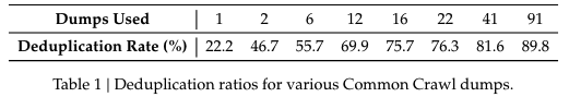
去重
使用了激进的去重策略, 扩大了去重的范围. 使用 MinhashLSH 算法, 在 document 和 string 两个粒度下进行去重. String 粒度是将 document 进行切分, 原始的 document 可以看做是一个 dump, 将一个 document 切分为多个 dumps. 实际证明, 当切分为 91 个 dumps 的时候, 去重的比例是使用 document 粒度去重比例的 4 倍.
严格去重策略, 保证了高质量数据的唯一性和完整性, 这在大规模数据集中特别重要.
过滤
过滤是对文本的质量进行评估, 这涉及到语言和语义的综合评估, 从单个样本, 以及整体样本的角度对数据质量进行评估, 移除低质量 web data. 对于高质量低资源的数据, 则不进行筛选.
过滤的手段主要包含:
- heuristic rules, 启发式规则
- models, 评估模型
通过各种手段, 移除有害有毒有争议的文本.
重新混合
在这个阶段, 通过数据的重新混合, 解决数据不平衡问题, 增加代表性不足领域的数据.
混合了 Internet text, math, code, books, 以及自己采集的数据. 在多样性之外, 还特别重视个人隐私和著作权的保护, 将侵犯隐私和知识产权的内容从数据集中移除.
总结
训练集共收集了 8.1T tokens.
训练超参数
初始化
标准差 0.006
优化器
AdamW. $\beta_1=0.9$, $\beta_2=0.95$, $\text{weight\_decay} = 0.1$
scheduler
- 2000 steps warmup steps
- cosine scheduler: 训练到 60% 的 tokens 时, 学习率下降到最大值的 0.316; 到 90% 的 tokens 时, 再下降到 60% 位置对应学习率的 0.316
- gradient clipping: 1.0
其他关键参数
- sequence length: 4096
- learning rate: 2.4e-4
- batch size: batch size scheduling strategy
- 在训练头 225B tokens 时, batch size 从 2304 逐渐增加到 9216
- 在剩余的训练过程中保持 9216 的大小
长上下文扩展
在预训练得到初始 4K 上下文长度版本的 DeepSeek-V2 后, 使用 YaRN 方法, 将上下文长度从 4K 扩展到 128K. 由于 MLA 中只有 $\mathbf{k}_t^R$ 中带有 RoPE 的位置信息, 所以 YaRN 也是施加到这个上面. 使用的 YaRN 参数为:
- scale $s=40$
- $\alpha=1$
- $\beta=32$
- target maximum context length = 160K
另外为了适配 MLA 机制, 调整了 length scaling factor, 因子 $\sqrt{t} = 0.0707 \ln s + 1$, 以最小化 perplexity.
YaRN 的方法需要训练. 训练了 1000 steps, 使用了 batch size 576, sequence length 32K. 尽管训练时基于 32K 的序列长度, 在 128K 长度上已经可以取得比较 robust 的效果了.
对齐训练
SFT
1.5M instances 的 instruction tuning datasets, 由 1.2M helpfulness instances 和 0.3M safety instances 组成. 加强了数据质量, 以减轻幻觉, 以及增强写作能力.
- SFT with 2 epochs
- learning rate 5e-6
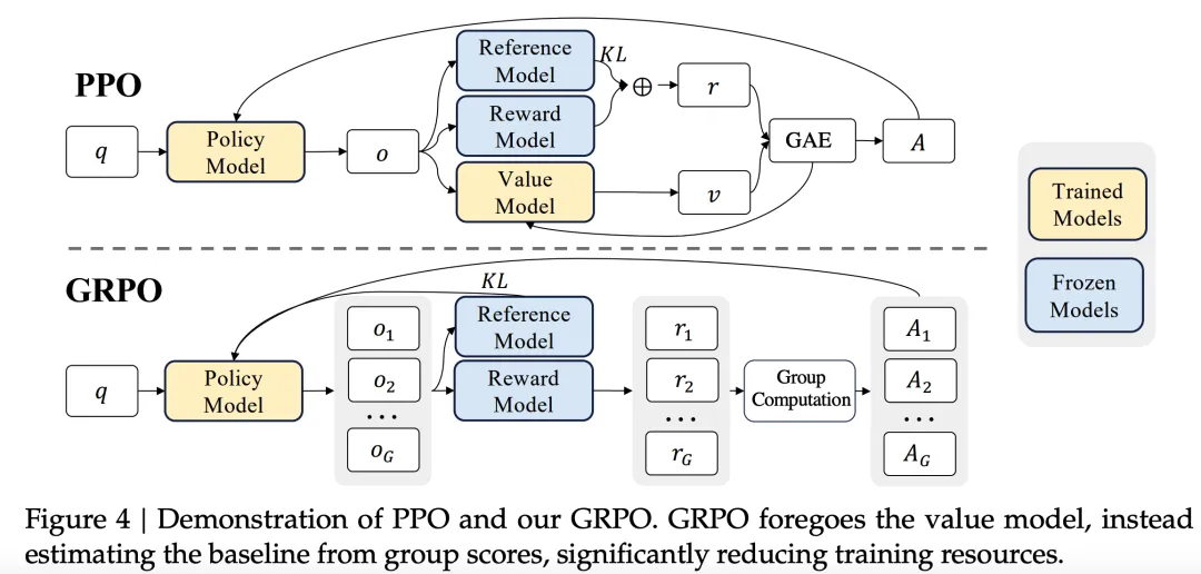
RL
DeepSeek-V2 没有使用 RM + PPO, 而是使用了 RM + GRPO 的方法. 相比之下, 这种方法不需要更新 policy 中的 value model 的方法.